HAWQ-V3: Dyadic Neural Network Quantization

1. Introduction

기존의 quantization 방식은 종종 simulated quantization을 사용했습니다. Simulated quantization은 파라미터를 quantized value로 저장하지만 inference 할 때는 floating point로 변경해서 연산을 수행합니다. 그래서 quantization을 통해서 모델 크기는 줄일 수 있었지만, inference 속도 향상은 되지 않았습니다. 이런 한계를 극복하기 위해 본 논문에서는 inference 할 때도 integer만 사용하고 integer division 연산도 bit shifting으로 대체하는 방법을 제시했습니다.

2. Proposed Method

2.1. Quantized Matrix Multiplication

Activation을 \(h\), weight를 \(W\)라고 가정하고, 각각을 quantization한 값을 \(q_h, q_w\), scale 값을 \(S_h, S_w\)라고 하면 activation과 weight를 행렬곱한 결과 \(a\)를 다음과 같이 나타낼 수 있습니다.

\[a=S_w S_h\left(q_w * q_h\right)\]

위처럼 계산한 결과를 다시 quantization해서 최종 output \(q_a\)를 다음과 같이 나타냅니다.

\[q_a=\operatorname{Int}\left(\frac{a}{S_a}\right)=\operatorname{Int}\left(\frac{S_w S_h}{S_a}\left(q_w * q_h\right)\right)\]

위의 식을 정리하면 \(q_w*q_h\)에서 INT4로 곱셈을 수행하고 INT32 precision으로 accumulation하는 방식으로 행렬곱하고 \(S_w S_h / S_a\)를 통해 scaling하는 방식으로 연산을 수행합니다. 여기서 scaling factor \(S_w S_h / S_a\)가 floating point가 돼서 \(q_w * q_h\)랑 곱해지면 floating point 연산이 수행이 되어버립니다.

본 논문에서는 scaling factor를 dyadic number로 치환해서 floating point 연산과 integer division 연산을 제거했습니다. Dyadic number는 \(b/2^c\) 형태로 표현되는 유리수인데, 이 형태로 표현하게 되면 integer multiplication과 bit shifting으로 scaling을 수행할 수 있습니다. 그래서 integer \(b, c\)를 통해 scaling factor를 다음과 같이 표현합니다.

\[b / 2^c=\mathrm{DN}\left(S_w S_h / S_a\right)\]

2.2. Batch Normalization

어떤 activation \(a\)에 Batch normalization을 적용하는 과정은 다음과 같습니다.

\[\mathrm{BN}(a)=\beta \frac{a-\mu_B}{\sigma_B}+\gamma\]

여기서 문제점은 BN parameter \(\mu_B, \sigma_B\)에 quantization을 적용하게 되면 accuracy 감소 문제가 심하게 발생합니다. 그래서 이전에 quantization 방법들은 BN parameter를 FP32 precision으로 저장했는데, 그런 방식은 accuracy 측면에서 도움이 되지만 integer-only hardware에는 적합하지 않습니다.

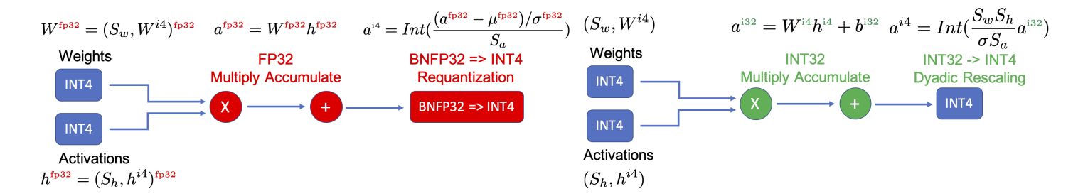
위의 그림에서 왼쪽은 fake quantization을 나타냅니다. weight과 bias는 INT4로 저장이 되었지만, 행렬곱을 할 때 FP32로 바뀌고 BN parameter도 FP32 형태로 저장을 합니다. 본 논문에서는 위의 오른쪽 그림처럼 convolution과 batch normalization을 합치는 과정을 수행합니다. BN의 standard deviation parameter가 scale factor랑 합쳐지고 mean parameter는 convolution 연산을 한 후에 bias 형태로 더해지게 됩니다. 이런 방식으로 BN 연산을 하면 모든 연산이 integer로 수행이 됩니다.

2.3. Residual Connection

Quantization은 linear하지 않기 때문에, residual connection에서 quantization을 적용하는 것은 문제가 발생할 가능성이 있습니다.

2.4. Mixed Precision and Integer Linear Programming

모든 layer를 같은 bit로 quantization하게 되면 accuracy가 급격히 감소하게 됩니다. 이를 보완하는 방법으로 precision에 민감한 layer는 높은 precision을 유지하고, 민감하지 않은 layer는 낮은 precision을 설정하는 방법이 있습니다. 하지만 hardware-specific metric을 기준으로 살펴보면 어떤 layer를 low precision으로 설정해도 latency 값이 감소하지 않을 가능성이 있습니다. 이런 경우에는 해당 layer가 precision에 민감하지 않더라도 높은 precision을 유지하는 게 좋습니다. 그래서 본 논문에서는 각 layer의 bit를 선택할 때 sensitivity 뿐만 아니라 hardware-specific metric을 고려해서 bit를 선택하는 방법을 Integer Linear Programming 형태로 제시합니다.

논문에서는 모델에 \(L\)개의 layer가 있고 각 layer마다 \(B\)개의 가능한 선택이 있다고 가정을 했습니다. 그리고 model perturbation, model size, BOPS(Bit Operations for calculating a layer)를 고려해서 최적화 문제를 다음과 같이 설계합니다.

\[\begin{aligned} \text { Objective: } & \min _{\left\{b_i\right\}_{i=1}^L} \sum_{i=1}^L \Omega_i^{\left(b_i\right)}, \\ \text { Subject to: } & \sum_{i=1}^L M_i^{\left(b_i\right)} \leq \text { Model Size Limit, } \\ & \sum_{i=1}^L G_i^{\left(b_i\right)} \leq \text { BOPS Limit, } \\ & \sum_{i=1}^L Q_i^{\left(b_i\right)} \leq \text { Latency Limit. } \end{aligned}\]

여기서 \(\Omega=\sum_{i=1}^L \Omega_i^{\left(b_i\right)}\)는 model perturbation을 의미하고, \(i\)번째 layer에 \(b_i\) bit를 선택했을 때 해당 layer의 perturbation을 \(\Omega_i^{\left(b_i\right)}\)로 표현합니다. 그리고 Hessian based perturbation (Dong et al., 2020) 방법을 사용해서 perturbation을 계산했습니다. \(M_i^{\left(b_i\right)}\) \(i\)번째 layer를 \(b_i\) bit로 quantization했을 때 크기, \(Q_i^{\left(b_i\right)}\)는 latency, \(G_i^{\left(b_i\right)}\)는 해당 layer를 계산하기 위한 BOPS를 의미하고 다음과 같이 계산합니다.

\[G_i^{\left(b_i\right)}=b_{w_i} b_{a_i} \mathrm{MAC}_i\]

\(\mathrm{MAC}_i\)는 \(i\)번째 layer의 Multiply-Accumulate operation의 개수이고, \(b_{w_i}, b_{a_i}\)는 weight과 activation의 bit precision입니다.

본 논문은 PULP library를 사용해서 ILP 문제를 sensitivity 값이 주어진 상황에서 1초 미만으로 해결했습니다. RL 기반의 다른 방법은 10시간 정도 소요되는 것에 비해 아주 빠르게 각 layer마다 적합한 bit를 찾습니다.

2.5. Hardware Deployment

모델의 efficiency (speed and energy consumption)을 측정할 때 model size 혹은 FLOPS만 고려해서는 안됩니다. 모델 크기 혹은 FLOPS 값이 작더라도 latency가 높고 에너지 소비가 많을 가능성이 있습니다. 왜냐하면 모델 크기 혹은 FLOPS에는 cache miss, data locality, memory bandwidth, underutilization of hardware 같은 요소가 반영되지 않기 때문입니다. 그래서 모델을 hardware에 직접 배포해서 latency를 측정하는 것이 중요합니다.

3. Result

ResNet50	InceptionV3
	!

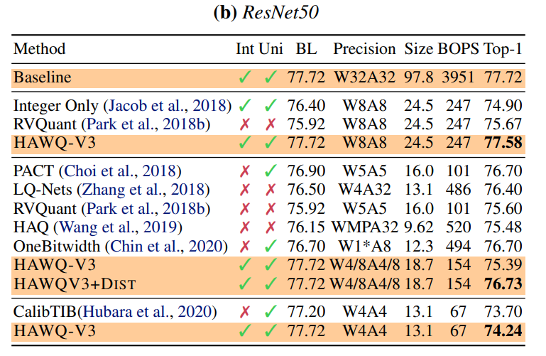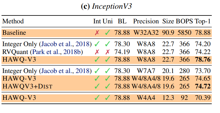위의 그림은 ImageNet으로 학습된 ResNet50, InceptionV3 모델에 논문에서 제시한 quantization 기법을 적용한 결과입니다. 8-bit quantization의 경우 기존의 다른 방법들보다 quantization 했을 때 Top-1 accuracy가 높고, quantization을 적용하지 않은 모델(baseline)과 많은 차이가 없습니다. Mixed precision의 경우 (W4/8A4/8)에도 기존의 다른 mixed precision 방법보다 Top-1 accuracy가 높습니다.